Data Science Methods for Forecasting in Energy and Economics

Jonathan Berrisch

University of Duisburg-Essen, House of Energy, Climate, and Finance

2025-06-30

Outline

\[ \newcommand{\A}{{\mathbb A}} \]

  Research Motivation

  Overview of the Thesis

  Online Aggregation

  Probabilistic Forecasting of European Carbon and Energy Prices

  Contributions

The beginning: June 2020

Artwork by @allison_horst

Motivation

	Energy market liberalization created complex, interconnected trading systems
	Renewable energy transition introduces uncertainty and volatility from weather-dependent generation
	Traditional point forecasts are inadequate for modern energy markets with increasing uncertainty
	Risk inherently is a probabilistic concept
	Probabilistic forecasting essential for risk management, planning and decision making in volatile energy environments
	Online learning methods needed for fast-updating models with streaming energy data

Image generated by Sora (OpenAI)

Overview of the Thesis

	Berrisch, J., & Ziel, F. (2023). CRPS learning. Journal of Econometrics, 237(2), 105221.
	Berrisch, J., & Ziel, F. (2024). Multivariate probabilistic CRPS learning with an application to day-ahead electricity prices. International Journal of Forecasting, 40(4), 1568–1586.
	Hirsch, S., Berrisch, J., & Ziel, F. (2024). Online Distributional Regression. arXiv preprint arXiv:2407.08750.
	Berrisch, J., & Ziel, F. (2022). Distributional modeling and forecasting of natural gas prices. Journal of Forecasting, 41(6), 1065–1086.
	Berrisch, J., Pappert, S., Ziel, F., & Arsova, A. (2023). Modeling volatility and dependence of European carbon and energy prices. Finance Research Letters, 52, 103503.
	Berrisch, J., Narajewski, M., & Ziel, F. (2023). High-resolution peak demand estimation using generalized additive models and deep neural networks. Energy and AI, 13, 100236.
	Berrisch, J. (2025). rcpptimer: Rcpp Tic-Toc Timer with OpenMP Support. arXiv preprint arXiv:2501.15856.

	Berrisch, J., & Ziel, F. (2023). CRPS learning. Journal of Econometrics, 237(2), 105221.
	Berrisch, J., & Ziel, F. (2024). Multivariate probabilistic CRPS learning with an application to day-ahead electricity prices. International Journal of Forecasting, 40(4), 1568–1586.
	Hirsch, S., Berrisch, J., & Ziel, F. (2024). Online Distributional Regression. arXiv preprint arXiv:2407.08750.
	Berrisch, J., & Ziel, F. (2022). Distributional modeling and forecasting of natural gas prices. Journal of Forecasting, 41(6), 1065–1086.
	Berrisch, J., Pappert, S., Ziel, F., & Arsova, A. (2023). Modeling volatility and dependence of European carbon and energy prices. Finance Research Letters, 52, 103503.
	Berrisch, J., Narajewski, M., & Ziel, F. (2023). High-resolution peak demand estimation using generalized additive models and deep neural networks. Energy and AI, 13, 100236.
	Berrisch, J. (2025). rcpptimer: Rcpp Tic-Toc Timer with OpenMP Support. arXiv preprint arXiv:2501.15856.

	Berrisch, J., & Ziel, F. (2023). CRPS learning. Journal of Econometrics, 237(2), 105221.
	Berrisch, J., & Ziel, F. (2024). Multivariate probabilistic CRPS learning with an application to day-ahead electricity prices. International Journal of Forecasting, 40(4), 1568–1586.
	Hirsch, S., Berrisch, J., & Ziel, F. (2024). Online Distributional Regression. arXiv preprint arXiv:2407.08750.
	Berrisch, J., & Ziel, F. (2022). Distributional modeling and forecasting of natural gas prices. Journal of Forecasting, 41(6), 1065–1086.
	Berrisch, J., Pappert, S., Ziel, F., & Arsova, A. (2023). Modeling volatility and dependence of European carbon and energy prices. Finance Research Letters, 52, 103503.
	Berrisch, J., Narajewski, M., & Ziel, F. (2023). High-resolution peak demand estimation using generalized additive models and deep neural networks. Energy and AI, 13, 100236.
	Berrisch, J. (2025). rcpptimer: Rcpp Tic-Toc Timer with OpenMP Support. arXiv preprint arXiv:2501.15856.

Overview

Online Distributional Regression

Distributional Modeling and Forecasting of Natural Gas Prices

Reduces estimation time by 2-3 orders of magnitude

Maintainins competitive forecasting accuracy

Real-World Validation in Energy Markets

Python Package ondil on Github and PyPi

Forecasting of Day-Ahead and Month-Ahead prices

To capture the full distribution of future prices

Extensive data analysis from 2011-2020

State-Space models, skewed Student’s t distribution

Python Package sstudentt on Github and PyPi

Overview

High-Resolution Peak Demand Estimation Using Generalized Additive Models and Deep Neural Networks

rcpptimer: Rcpp Tic-Toc Timer with OpenMP Support

Predict high-resolution electricity peaks using only low-resolution data

Combine GAMs and DNN’s for superior accuracy

Won Western Power Distribution Competition

Won Best-Student-Presentation Award

R Package rcpptimer on Github and CRAN

Provides Rcpp bindings for cpptimer

tic-toc class for timing C++ code

Supports nested, overlapping and scoped timers

Supports OpenMP parallelism

//[[Rcpp::depends(rcpptimer)]]
#include <rcpptimer.h>

void main(){
  Rcpp::Timer timer;
  Rcpp::Timer::ScopedTimer _(timer, "ST");

  timer.tic();
  // Some more code
  timer.toc();
} // ScopedTimer will stop automatically

CRPS Learning

Berrisch, J., & Ziel, F. (2023). Journal of Econometrics, 237(2), 105221.

Introduction

The Idea:

• Combine multiple forecasts instead of choosing one

• Combination weights may vary over time, over the distribution or both

2 Popular options for combining distributions:

• Combining across quantiles (this paper)
  • Horizontal aggregation, vincentization
• Combining across probabilities
  • Vertical aggregation

• Time
• Distribution

The Framework of Prediction under Expert Advice

The sequential framework

Each day, \(t = 1, 2, ... T\)

• The forecaster receives predictions \(\widehat{X}_{t,k}\) from \(K\) experts
• The forecaster assings weights \(w_{t,k}\) to each expert
• The forecaster calculates her prediction: \[\begin{equation} \widetilde{X}_{t} = \sum_{k=1}^K w_{t,k} \widehat{X}_{t,k}. \label{eq_forecast_def} \end{equation}\]
• The realization for \(t\) is observed

• The experts can be institutions, persons, or models
• The forecasts can be point-forecasts (i.e., mean or median) or full predictive distributions
• We do not need any assumptions concerning the underlying data
• Cesa-Bianchi & Lugosi (2006)

The Regret

Weights are updated sequentially according to the past performance of the \(K\) experts.

That is, a loss function \(\ell\) is needed. This is used to compute the cumulative regret \(R_{t,k}\)

\[\begin{equation} R_{t,k} = \widetilde{L}_{t} - \widehat{L}_{t,k} = \sum_{i = 1}^t \ell(\widetilde{X}_{i},Y_i) - \ell(\widehat{X}_{i,k},Y_i)\label{eq:regret} \end{equation}\]

The cumulative regret:

• Indicates the predictive accuracy of the expert \(k\) until time \(t\).
• Measures how much the forecaster regrets not having followed the expert’s advice

Popular loss functions for point forecasting Gneiting (2011):

\(\ell_2\) loss:

\[\begin{equation} \ell_2(x, y) = | x -y|^2 \label{eq:elltwo} \end{equation}\]

Strictly proper for mean prediction

\(\ell_1\) loss:

\[\begin{equation} \ell_1(x, y) = | x -y| \label{eq:ellone} \end{equation}\]

Strictly proper for median predictions

Popular Algorithms and the Risk

Popular Aggregation Algorithms

The naive combination

\[\begin{equation} w_{t,k}^{\text{Naive}} = \frac{1}{K}\label{eq:naive_combination} \end{equation}\]

The exponentially weighted average forecaster (EWA)

\[\begin{equation} \begin{aligned} w_{t,k}^{\text{EWA}} & = \frac{e^{\eta R_{t,k}} }{\sum_{k = 1}^K e^{\eta R_{t,k}}}\\ & = \frac{e^{-\eta \ell(\widehat{X}_{t,k},Y_t)} w^{\text{EWA}}_{t-1,k} }{\sum_{k = 1}^K e^{-\eta \ell(\widehat{X}_{t,k},Y_t)} w^{\text{EWA}}_{t-1,k}} \end{aligned}\label{eq:exp_combination} \end{equation}\]

Optimality

In stochastic settings, the cumulative Risk should be analyzed Wintenberger (2017): \[\begin{align} &\underbrace{\widetilde{\mathcal{R}}_t = \sum_{i=1}^t \mathbb{E}[\ell(\widetilde{X}_{i},Y_i)|\mathcal{F}_{i-1}]}_{\text{Cumulative Risk of Forecaster}} \\ &\underbrace{\widehat{\mathcal{R}}_{t,k} = \sum_{i=1}^t \mathbb{E}[\ell(\widehat{X}_{i,k},Y_i)|\mathcal{F}_{i-1}]}_{\text{Cumulative Risk of Experts}} \label{eq_def_cumrisk} \end{align}\]

Optimal Convergence

The selection problem

\[\begin{equation} \frac{1}{t}\left(\widetilde{\mathcal{R}}_t - \widehat{\mathcal{R}}_{t,\min} \right) \stackrel{t\to \infty}{\rightarrow} a \quad \text{with} \quad a \leq 0. \label{eq_opt_select} \end{equation}\] The forecaster is asymptotically not worse than the best expert \(\widehat{\mathcal{R}}_{t,\min}\).

The convex aggregation problem

\[\begin{equation} \frac{1}{t}\left(\widetilde{\mathcal{R}}_t - \widehat{\mathcal{R}}_{t,\pi} \right) \stackrel{t\to \infty}{\rightarrow} b \quad \text{with} \quad b \leq 0 . \label{eq_opt_conv} \end{equation}\] The forecaster is asymptotically not worse than the best convex combination \(\widehat{X}_{t,\pi}\) in hindsight (oracle).

Optimal rates with respect to selection \(\eqref{eq_opt_select}\) and convex aggregation \(\eqref{eq_opt_conv}\) Wintenberger (2017):

\[\begin{align} \frac{1}{t}\left(\widetilde{\mathcal{R}}_t - \widehat{\mathcal{R}}_{t,\min} \right) & = \mathcal{O}\left(\frac{\log(K)}{t}\right)\label{eq_optp_select} \end{align}\]

\[\begin{align} \frac{1}{t}\left(\widetilde{\mathcal{R}}_t - \widehat{\mathcal{R}}_{t,\pi} \right) & = \mathcal{O}\left(\sqrt{\frac{\log(K)}{t}}\right) \label{eq_optp_conv} \end{align}\]

Algorithms can statisfy both \(\eqref{eq_optp_select}\) and \(\eqref{eq_optp_conv}\) depending on:

• The loss function
• Regularity conditions on \(Y_t\) and \(\widehat{X}_{t,k}\)
• The weighting scheme

Optimal Convergence

EWA satisfies optimal selection convergence \(\eqref{eq_optp_select}\) in a deterministic setting if:

• Loss \(\ell\) is exp-concave
• Learning-rate \(\eta\) is chosen correctly

Those results can be converted to any stochastic setting Wintenberger (2017).

Optimal convex aggregation convergence \(\eqref{eq_optp_conv}\) can be satisfied by applying the kernel-trick:

\[\begin{align} \ell^{\nabla}(x,y) = \ell'(\widetilde{X},y) x \end{align}\]

\(\ell'\) is the subgradient of \(\ell\) at forecast combination \(\widetilde{X}\).

Probabilistic Setting

An appropriate choice:

\[\begin{equation*} \text{CRPS}(F, y) = \int_{\mathbb{R}} {(F(x) - \mathbb{1}\{ x > y \})}^2 dx \label{eq:crps} \end{equation*}\]

It’s strictly proper Gneiting & Raftery (2007).

Using the CRPS, we can calculate time-adaptive weights \(w_{t,k}\). However, what if the experts’ performance varies in parts of the distribution?

Utilize this relation:

\[\begin{equation*} \text{CRPS}(F, y) = 2 \int_0^{1} \text{QL}_p(F^{-1}(p), y) dp.\label{eq_crps_qs} \end{equation*}\]

… to combine quantiles of the probabilistic forecasts individually using the quantile-loss QL.

CRPS Learning Optimality

• Almost Optimal Convergence
• Conditions + Lemma
• Proposition + Theorem

QL is convex, but not exp-concave

Bernstein Online Aggregation (BOA) lets us weaken the exp-concavity condition. It satisfies that there exist a \(C>0\) such that for \(x>0\) it holds that

\[\begin{equation} P\left( \frac{1}{t}\left(\widetilde{\mathcal{R}}_t - \widehat{\mathcal{R}}_{t,\pi} \right) \leq C \log(\log(t)) \left(\sqrt{\frac{\log(K)}{t}} + \frac{\log(K)+x}{t}\right) \right) \geq 1-e^{-x} \label{eq_boa_opt_conv} \end{equation}\]

Almost optimal w.r.t. convex aggregation \(\eqref{eq_optp_conv}\) Wintenberger (2017).

The same algorithm satisfies that there exist a \(C>0\) such that for \(x>0\) it holds that \[\begin{equation} P\left( \frac{1}{t}\left(\widetilde{\mathcal{R}}_t - \widehat{\mathcal{R}}_{t,\min} \right) \leq C\left(\frac{\log(K)+\log(\log(Gt))+ x}{\alpha t}\right)^{\frac{1}{2-\beta}} \right) \geq 1-2e^{-x} \label{eq_boa_opt_select} \end{equation}\]

if \(Y_t\) is bounded, the considered loss \(\ell\) is convex \(G\)-Lipschitz and weak exp-concave in its first coordinate.

Almost optimal w.r.t. selection \(\eqref{eq_optp_select}\) Gaillard & Wintenberger (2018).

We show that this holds for QL under feasible conditions.

Lemma 1

\[\begin{align} 2\overline{\widehat{\mathcal{R}}}^{\text{QL}}_{t,\min} & \leq \widehat{\mathcal{R}}^{\text{CRPS}}_{t,\min} \label{eq_risk_ql_crps_expert} \\ 2\overline{\widehat{\mathcal{R}}}^{\text{QL}}_{t,\pi} & \leq \widehat{\mathcal{R}}^{\text{CRPS}}_{t,\pi} . \label{eq_risk_ql_crps_convex} \end{align}\]

Pointwise can outperform constant procedures

QL is convex but not exp-concave:

Almost optimal convergence w.r.t. convex aggregation \(\eqref{eq_boa_opt_conv}\)

For almost optimal congerence w.r.t. selection \(\eqref{eq_boa_opt_select}\) we need to check A1 and A2:

QL is Lipschitz continuous:

A1 holds

A1

For some \(G>0\) it holds for all \(x_1,x_2\in \mathbb{R}\) and \(t>0\) that

\[ | \ell(x_1, Y_t)-\ell(x_2, Y_t) | \leq G |x_1-x_2|\]

A2 For some \(\alpha>0\), \(\beta\in[0,1]\) it holds for all \(x_1,x_2 \in \mathbb{R}\) and \(t>0\) that

\[\begin{align*} \mathbb{E}[ & \ell(x_1, Y_t)-\ell(x_2, Y_t) | \mathcal{F}_{t-1}] \leq \\ & \mathbb{E}[ \ell'(x_1, Y_t)(x_1 - x_2) |\mathcal{F}_{t-1}] \\ & + \mathbb{E}\left[ \left. \left( \alpha(\ell'(x_1, Y_t)(x_1 - x_2))^{2}\right)^{1/\beta} \right|\mathcal{F}_{t-1}\right] \end{align*}\]

Almost optimal w.r.t. selection \(\eqref{eq_optp_select}\) Gaillard & Wintenberger (2018).

Conditional quantile risk: \(\mathcal{Q}_p(x) = \mathbb{E}[ \text{QL}_p(x, Y_t) | \mathcal{F}_{t-1}]\).

convexity properties of \(\mathcal{Q}_p\) depend on the conditional distribution \(Y_t|\mathcal{F}_{t-1}\).

Proposition 1

Let \(Y\) be a univariate random variable with (Radon-Nikodym) \(\nu\)-density \(f\), then for the second subderivative of the quantile risk \(\mathcal{Q}_p(x) = \mathbb{E}[ \text{QL}_p(x, Y) ]\) of \(Y\) it holds for all \(p\in(0,1)\) that \(\mathcal{Q}_p'' = f.\) Additionally, if \(f\) is a continuous Lebesgue-density with \(f\geq\gamma>0\) for some constant \(\gamma>0\) on its support \(\text{spt}(f)\) then is \(\mathcal{Q}_p\) is \(\gamma\)-strongly convex.

Strong convexity with \(\beta=1\) implies weak exp-concavity A2 Gaillard & Wintenberger (2018)

A1 and A2 give us almost optimal convergence w.r.t. selection \(\eqref{eq_boa_opt_select}\)

Theorem 1

The gradient based fully adaptive Bernstein online aggregation (BOAG) applied pointwise for all \(p\in(0,1)\) on \(\text{QL}\) satisfies \(\eqref{eq_boa_opt_conv}\) with minimal CRPS given by

\[\widehat{\mathcal{R}}_{t,\pi} = 2\overline{\widehat{\mathcal{R}}}^{\text{QL}}_{t,\pi}.\]

If \(Y_t|\mathcal{F}_{t-1}\) is bounded and has a pdf \(f_t\) satifying \(f_t>\gamma >0\) on its support \(\text{spt}(f_t)\) then \(\ref{eq_boa_opt_select}\) holds with \(\beta=1\) and

\[\widehat{\mathcal{R}}_{t,\min} = 2\overline{\widehat{\mathcal{R}}}^{\text{QL}}_{t,\min}\].

We apply Bernstein Online Aggregation (BOA). It lets us weaken the exp-concavity condition while almost keeping the optimalities \(\ref{eq_optp_select}\) and \(\ref{eq_optp_conv}\).

A Probabilistic Example

Simple Example:

\[\begin{align} Y_t & \sim \mathcal{N}(0,\,1) \\ \widehat{X}_{t,1} & \sim \widehat{F}_{1} = \mathcal{N}(-1,\,1) \\ \widehat{X}_{t,2} & \sim \widehat{F}_{2} = \mathcal{N}(3,\,4) \label{eq:dgp_sim1} \end{align}\]

• True weights vary over \(p\)
• Figures show the ECDF and calculated weights using \(T=25\) realizations
• Pointwise solution creates rough estimates
• Pointwise is better than constant
• Smooth solution is better than pointwise

• CDFs
• Weights

The Smoothing Procedures

• Penalized Smoothing
• Basis Smoothing

Penalized cubic B-Splines for smoothing weights:

Let \(\varphi=(\varphi_1,\ldots, \varphi_L)\) be bounded basis functions on \((0,1)\) Then we approximate \(w_{t,k}\) by

\[\begin{align} w_{t,k}^{\text{smooth}} = \sum_{l=1}^L \beta_l \varphi_l = \beta'\varphi \end{align}\]

with parameter vector \(\beta\). The latter is estimated to penalize \(L_2\)-smoothing which minimizes

\[\begin{equation} \| w_{t,k} - \beta' \varphi \|^2_2 + \lambda \| \mathcal{D}^{d} (\beta' \varphi) \|^2_2 \label{eq_function_smooth} \end{equation}\]

with differential operator \(\mathcal{D}\)

Computation is easy, since we have an analytical solution

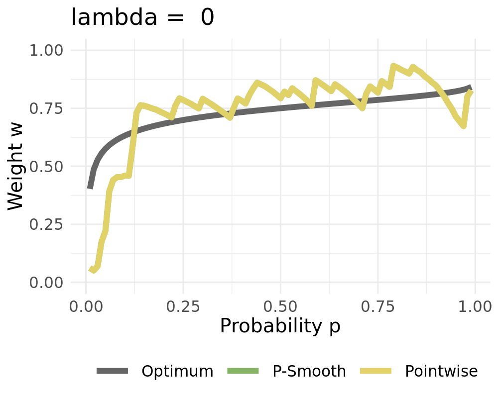
We receive the constant solution for high values of \(\lambda\) when setting \(d=1\)

Represent weights as linear combinations of bounded basis functions:

\[\begin{equation} w_{t,k} = \sum_{l=1}^L \beta_{t,k,l} \varphi_l = \boldsymbol \beta_{t,k}' \boldsymbol \varphi \end{equation}\]

A popular choice are are B-Splines as local basis functions

\(\boldsymbol \beta_{t,k}\) is calculated using a reduced regret matrix:

\[\begin{equation} \underbrace{\boldsymbol r_{t}}_{\text{LxK}} = \frac{L}{P} \underbrace{\boldsymbol B'}_{\text{LxP}} \underbrace{\left({\boldsymbol{QL}}_{\mathcal{P}}^{\nabla}(\widetilde{\boldsymbol X}_{t},Y_t)- {\boldsymbol{QL}}_{\mathcal{P}}^{\nabla}(\widehat{\boldsymbol X}_{t},Y_t)\right)}_{\text{PxK}} \end{equation}\]

\(\boldsymbol r_{t}\) is transformed from PxK to LxK

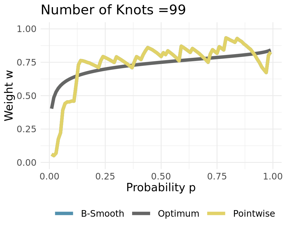
If \(L = P\) it holds that \(\boldsymbol \varphi = \boldsymbol{I}\) For \(L = 1\) we receive constant weights

Weights converge to the constant solution if \(L\rightarrow 1\)

The Proposed CRPS-Learning Algorithm

Initialization:

Array of expert predicitons: \(\widehat{X}_{t,p,k}\)

Vector of Prediction targets: \(Y_t\)

Starting Weights: \(\boldsymbol w_0=(w_{0,1},\ldots, w_{0,K})\)

Penalization parameter: \(\lambda\geq 0\)

B-spline and penalty matrices \(\boldsymbol B\) and \(\boldsymbol D\) on \(\mathcal{P}= (p_1,\ldots,p_M)\)

Hat matrix: \[\boldsymbol{\mathcal{H}} = \boldsymbol B(\boldsymbol B'\boldsymbol B+ \lambda (\alpha \boldsymbol D_1'\boldsymbol D_1 + (1-\alpha) \boldsymbol D_2'\boldsymbol D_2))^{-1} \boldsymbol B'\]

Cumulative Regret: \(R_{0,k} = 0\)

Range parameter: \(E_{0,k}=0\)

Starting pseudo-weights: \(\boldsymbol \beta_0 = \boldsymbol B^{\text{pinv}}\boldsymbol w_0(\boldsymbol{\mathcal{P}})\)

Core:

for( t in 1:T ) {

    \(\widetilde{\boldsymbol X}_{t} = \text{Sort}\left( \boldsymbol w_{t-1}'(\boldsymbol P) \widehat{\boldsymbol X}_{t} \right)\) # Prediction

    \(\boldsymbol r_{t} = \frac{L}{M} \boldsymbol B' \left({\boldsymbol{QL}}_{\boldsymbol{\mathcal P}}^{\nabla}(\widetilde{\boldsymbol X}_{t},Y_t)- {\boldsymbol{QL}}_{\boldsymbol{\mathcal P}}^{\nabla}(\widehat{\boldsymbol X}_{t},Y_t)\right)\)

    \(\boldsymbol E_{t} = \max(\boldsymbol E_{t-1}, \boldsymbol r_{t}^+ + \boldsymbol r_{t}^-)\)

    \(\boldsymbol V_{t} = \boldsymbol V_{t-1} + \boldsymbol r_{t}^{ \odot 2}\)

    \(\boldsymbol \eta_{t} =\min\left( \left(-\log(\boldsymbol \beta_{0}) \odot \boldsymbol V_{t}^{\odot -1} \right)^{\odot\frac{1}{2}} , \frac{1}{2}\boldsymbol E_{t}^{\odot-1}\right)\)

    \(\boldsymbol R_{t} = \boldsymbol R_{t-1}+ \boldsymbol r_{t} \odot \left( \boldsymbol 1 - \boldsymbol \eta_{t} \odot \boldsymbol r_{t} \right)/2 + \boldsymbol E_{t} \odot \mathbb{1}\{-2\boldsymbol \eta_{t}\odot \boldsymbol r_{t} > 1\}\)

    \(\boldsymbol \beta_{t} = K \boldsymbol \beta_{0} \odot \boldsymbol {SoftMax}\left( - \boldsymbol \eta_{t} \odot \boldsymbol R_{t} + \log( \boldsymbol \eta_{t}) \right)\)

    \(\boldsymbol w_{t}(\boldsymbol P) = \underbrace{\boldsymbol B(\boldsymbol B'\boldsymbol B+ \lambda (\alpha \boldsymbol D_1'\boldsymbol D_1 + (1-\alpha) \boldsymbol D_2'\boldsymbol D_2))^{-1} \boldsymbol B'}_{\boldsymbol{\mathcal{H}}} \boldsymbol B \boldsymbol \beta_{t}\)

}

Simulation Study

• BOA
• Comparison to EWA and ML-Poly
• Study Forget

Data Generating Process of the simple probabilistic example:

\[\begin{align*} Y_t &\sim \mathcal{N}(0,\,1)\\ \widehat{X}_{t,1} &\sim \widehat{F}_{1}=\mathcal{N}(-1,\,1) \\ \widehat{X}_{t,2} &\sim \widehat{F}_{2}=\mathcal{N}(3,\,4) \end{align*}\]

• Constant solution \(\lambda \rightarrow \infty\)
• Pointwise Solution of the proposed BOAG
• Smoothed Solution of the proposed BOAG
  • Weights are smoothed during learning
  • Smooth weights are used to calculate Regret, adjust weights, etc.

• QL Deviation
• CRPS vs. Lambda
• Knots

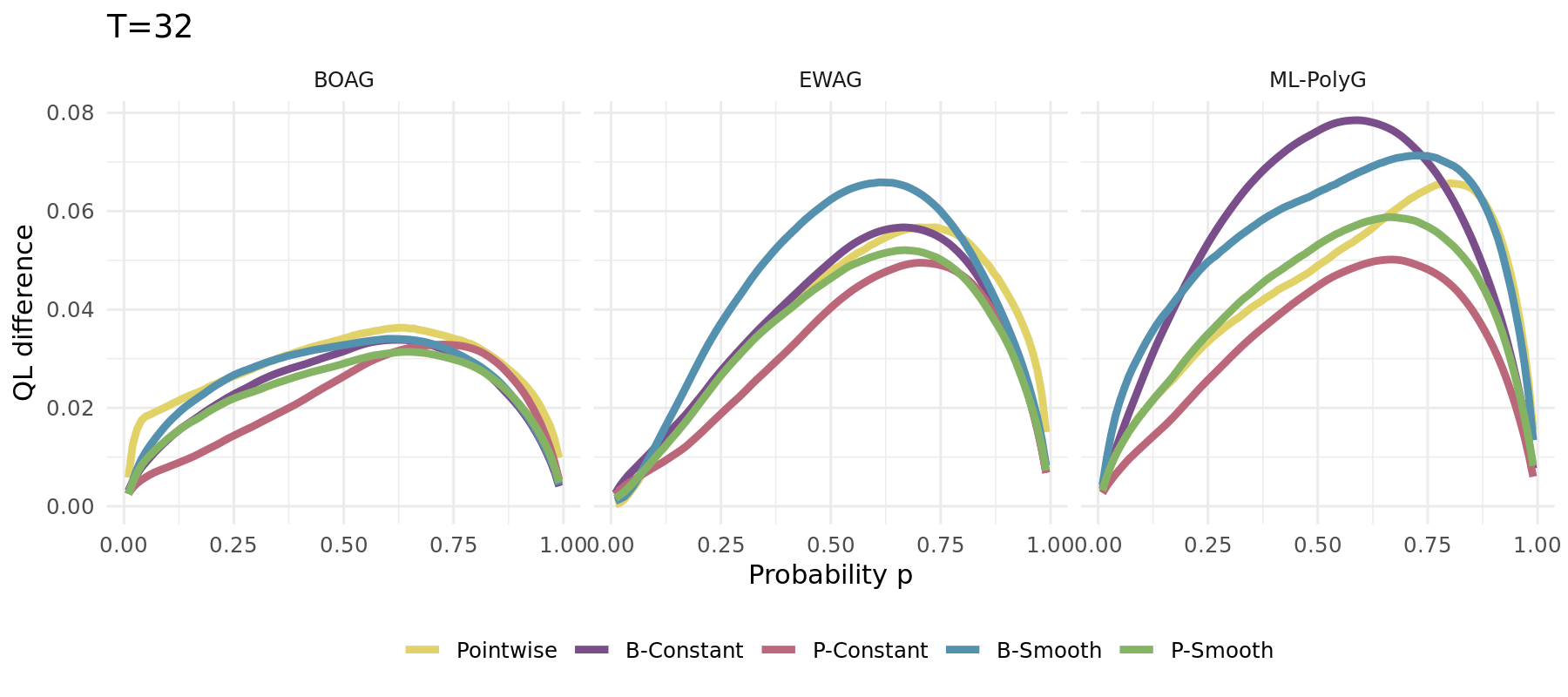
Deviation from best attainable QL (1000 runs).

CRPS Values for different \(\lambda\) (1000 runs)

CRPS for different number of knots (1000 runs)

The same simulation carried out for different algorithms (1000 runs):

New DGP:

\[\begin{align*} Y_t &\sim \mathcal{N}\left(\frac{\sin(0.005 \pi t )}{2},\,1\right) \\ \widehat{X}_{t,1} &\sim \widehat{F}_{1} = \mathcal{N}(-1,\,1) \\ \widehat{X}_{t,2} &\sim \widehat{F}_{2} = \mathcal{N}(3,\,4) \end{align*}\]

Changing optimal weights

Single run example depicted aside

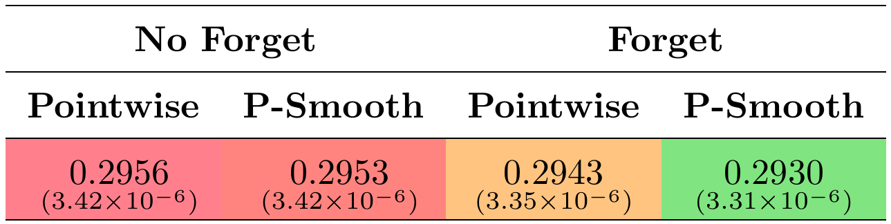
No forgetting leads to long-term constant weights

 

Application Study

• Overview
• Experts
• Results

Data:

• Forecasting European emission allowances (EUA)
• Daily month-ahead prices
• Jan 13 - Dec 20 (Phase III, 2092 Obs)
• Rolling Window (length 250 ~ 1 year)

Combination methods:

• Online
  • Naive, BOAG, EWAG, ML-PolyG, BMA
• Batch
  • QRlin, QRconv

Tuning paramter grids:

• Smoothing Penalty: \(\Lambda= \{0\}\cup \{2^x|x\in \{-4,-3.5,\ldots,12\}\}\)
• Learning Rates: \(\mathcal{E}= \{2^x|x\in \{-1,-0.5,\ldots,9\}\}\)

Simple exponential smoothing with additive errors (ETS-ANN):

\[\begin{align*} Y_{t} = l_{t-1} + \varepsilon_t \quad \text{with} \quad l_t = l_{t-1} + \alpha \varepsilon_t \quad \text{and} \quad \varepsilon_t \sim \mathcal{N}(0,\sigma^2) \end{align*}\]

Quantile regression (QuantReg): For each \(p \in \mathcal{P}\) we assume:

\[\begin{align*} F^{-1}_{Y_t}(p) = \beta_{p,0} + \beta_{p,1} Y_{t-1} + \beta_{p,2} |Y_{t-1}-Y_{t-2}| \end{align*}\]

ARIMA(1,0,1)-GARCH(1,1) with Gaussian errors (ARMA-GARCH):

\[\begin{align*} Y_{t} = \mu + \phi(Y_{t-1}-\mu) + \theta \varepsilon_{t-1} + \varepsilon_t \quad \text{with} \quad \varepsilon_t = \sigma_t Z, \quad \sigma_t^2 = \omega + \alpha \varepsilon_{t-1}^2 + \beta \sigma_{t-1}^2 \quad \text{and} \quad Z_t \sim \mathcal{N}(0,1) \end{align*}\]

ARIMA(0,1,0)-I-EGARCH(1,1) with Gaussian errors (I-EGARCH):

\[\begin{align*} Y_{t} = \mu + Y_{t-1} + \varepsilon_t \quad \text{with} \quad \varepsilon_t = \sigma_t Z, \quad \log(\sigma_t^2) = \omega + \alpha Z_{t-1}+ \gamma (|Z_{t-1}|-\mathbb{E}|Z_{t-1}|) + \beta \log(\sigma_{t-1}^2) \quad \text{and} \quad Z_t \sim \mathcal{N}(0,1) \end{align*}\]

ARIMA(0,1,0)-GARCH(1,1) with student-t errors (I-GARCHt):

\[\begin{align*} Y_{t} = \mu + Y_{t-1} + \varepsilon_t \quad \text{with} \quad \varepsilon_t = \sigma_t Z, \quad \sigma_t^2 = \omega + \alpha \varepsilon_{t-1}^2 + \beta \sigma_{t-1}^2 \quad \text{and} \quad Z_t \sim t(0,1, \nu) \end{align*}\]

• Significance
• QL
• Cumulative Loss Difference
• Weights (BOAG P-Smooth)
• Weights (Last)

ETS	QuantReg	ARMA-GARCH	I-EGARCH	I-GARCHt
2.101(>.999)	1.358(>.999)	0.52(0.993)	0.511(0.999)	-0.037(0.406)

	BOAG	EWAG	ML-PolyG	BMA	QRlin	QRconv
Pointwise	-0.170(0.055)	-0.089(0.175)	-0.141(0.112)	0.032(0.771)	3.482(>.999)	-0.019(0.309)
B-Constant	-0.118(0.146)	-0.049(0.305)	-0.090(0.218)	0.038(0.834)	4.002(>.999)	0.539(0.996)
P-Constant	-0.138(0.020)	-0.070(0.137)	-0.133(0.026)	0.039(0.851)	5.275(>.999)	0.009(0.683)
B-Smooth	-0.173(0.062)	-0.065(0.276)	-0.141(0.118)	-0.042(0.386)	-	-
P-Smooth	-0.182(0.039)	-0.107(0.121)	-0.160(0.065)	0.040(0.804)	3.495(>.999)	-0.012(0.369)

CRPS difference to Naive. Negative values correspond to better performance (the best value is bold).
Additionally, we show the p-value of the DM-test, testing against Naive. The cells are colored with respect to their values (the greener better).

Multivariate Probabilistic CRPS Learning with an Application to Day-Ahead Electricity Prices

Berrisch, J., & Ziel, F. (2024). International Journal of Forecasting, 40(4), 1568-1586.

Multivariate CRPS Learning

We extend the B-Smooth and P-Smooth procedures to the multivariate setting:

• Penalized Smoothing
• Basis Smoothing

Let \(\boldsymbol{\psi}^{\text{mv}}=(\psi_1,\ldots, \psi_{D})\) and \(\boldsymbol{\psi}^{\text{pr}}=(\psi_1,\ldots, \psi_{P})\) be two sets of bounded basis functions on \((0,1)\):

\[\begin{equation*} \boldsymbol w_{t,k} = \boldsymbol{\psi}^{\text{mv}} \boldsymbol{b}_{t,k} {\boldsymbol{\psi}^{pr}}' \end{equation*}\]

with parameter matix \(\boldsymbol b_{t,k}\). The latter is estimated to penalize \(L_2\)-smoothing which minimizes

\[\begin{align} & \| \boldsymbol{\beta}_{t,d, k}' \boldsymbol{\varphi}^{\text{pr}} - \boldsymbol b_{t, d, k}' \boldsymbol{\psi}^{\text{pr}} \|^2_2 + \lambda^{\text{pr}} \| \mathcal{D}_{q} (\boldsymbol b_{t, d, k}' \boldsymbol{\psi}^{\text{pr}}) \|^2_2 + \nonumber \\ & \| \boldsymbol{\beta}_{t, p, k}' \boldsymbol{\varphi}^{\text{mv}} - \boldsymbol b_{t, p, k}' \boldsymbol{\psi}^{\text{mv}} \|^2_2 + \lambda^{\text{mv}} \| \mathcal{D}_{q} (\boldsymbol b_{t, p, k}' \boldsymbol{\psi}^{\text{mv}}) \|^2_2 \nonumber \end{align}\]

with differential operator \(\mathcal{D}_q\) of order \(q\)

We have an analytical solution.

Linear combinations of bounded basis functions:

\[\begin{equation} \underbrace{\boldsymbol w_{t,k}}_{D \text{ x } P} = \sum_{j=1}^{\widetilde D} \sum_{l=1}^{\widetilde P} \beta_{t,j,l,k} \varphi^{\text{mv}}_{j} \varphi^{\text{pr}}_{l} = \underbrace{\boldsymbol \varphi^{\text{mv}}}_{D\text{ x }\widetilde D} \boldsymbol \beta_{t,k} \underbrace{{\boldsymbol\varphi^{\text{pr}}}'}_{\widetilde P \text{ x }P} \nonumber \end{equation}\]

A popular choice: B-Splines

\(\boldsymbol \beta_{t,k}\) is calculated using a reduced regret matrix:

\(\underbrace{\boldsymbol r_{t,k}}_{\widetilde P \times \widetilde D} = \boldsymbol \varphi^{\text{pr}} \underbrace{\left({\boldsymbol{QL}}_{\mathcal{P}}^{\nabla}(\widetilde{\boldsymbol X}_{t},Y_t)- {\boldsymbol{QL}}_{\mathcal{P}}^{\nabla}(\widehat{\boldsymbol X}_{t},Y_t)\right)}_{\text{PxD}}\boldsymbol \varphi^{\text{mv}}\)

If \(\widetilde P = P\) it holds that \(\boldsymbol \varphi^{pr} = \boldsymbol{I}\) (pointwise)

For \(\widetilde P = 1\) we receive constant weights

Application

Data

• Day-Ahead electricity price forecasts from Marcjasz et al. (2023)
• Produced using probabilistic neural networks
• 24-dimensional distributional forecasts
• Distribution assumptions: JSU and Normal
• 8 experts (4 JSU, 4 Normal)
• 27th Dec. 2018 to 31st Dec. 2020 (736 days)
• We extract 99 quantiles (percentiles)

Setup

Evaluation: Exclude first 182 observations

Extensions: Penalized smoothing | Forgetting

Tuning strategies:

• Bayesian Fix
  • Sophisticated Baesian Search algorithm
• Online
  • Dynamic based on past performance
• Bayesian Online
  • First Bayesian Fix then Online

Computation Time: ~30 Minutes

Results

JSU1	JSU2	JSU3	JSU4	Norm1	Norm2	Norm3	Norm4	Naive
1.487	1.444	1.499	1.374	1.414	1.535	1.420	1.422	1.295

Description	Parameter Tuning	BOA	ML-Poly	EWA
Constant		1.2933	1.2966	1.3188
Pointwise		1.2936	1.3010	1.3101
FTL		1.3752	1.3692	1.3863
B Constant Pr		1.2936	1.3000	1.3432
B Constant Mv		1.2918	1.2945	1.3076
Forget	Bayesian Fix	1.2930	1.2956	1.3096
Full	Bayesian Fix	1.2905	1.2902	1.2870.
Smooth.forget	Bayesian Fix	1.2911	1.2912	1.2869.
Smooth	Bayesian Fix	1.2918	1.2917	1.2873.
Forget	Bayesian Online	1.2855**	1.2961	1.3098
Full	Bayesian Online	1.2919	1.2873.	1.2873.
Smooth.forget	Bayesian Online	1.2845**	1.2862*	1.2864.
Smooth	Bayesian Online	1.2918	1.2918	1.2874.
Forget	Sampling Online	1.2855**	1.2961	1.3114
Full	Sampling Online	1.2886	1.2861*	1.2873.
Smooth.forget	Sampling Online	1.2845***	1.2867*	1.2866.
Smooth	Sampling Online	1.2918	1.2917	1.2877.

Coloring w.r.t. test statistic: <-5 -4 -3 -2 -1 0 1 2 3 4 >5

Significance denoted by: . p < 0.1; * p < 0.05; ** p < 0.01; *** p < 0.001;

• Constant
• Pointwise
• B Constant PR
• B Constant MV
• Smooth.Forget

Results

• Chosen Parameters
• Weights: Hour 16:00-17:00
• Weights: Median

Non-Equidistant Knots

• Knot Placement Illustration
• Knot Placement Details

d3 = require("d3@7")

bsplineData = FileAttachment("assets/mcrps_learning/basis_functions.csv").csv({ typed: true })

function updateChartInner(g, x, y, linesGroup, color, line, data) {
  // Update axes with transitions
  x.domain([0, d3.max(data, d => d.x)]);
  g.select(".x-axis").transition().duration(1500).call(d3.axisBottom(x).ticks(10));
  y.domain([0, d3.max(data, d => d.y)]);
  g.select(".y-axis").transition().duration(1500).call(d3.axisLeft(y).ticks(5));

  // Group data by basis function
  const dataByFunction = Array.from(d3.group(data, d => d.b));
  const keyFn = d => d[0];

  // Update basis function lines
  const u = linesGroup.selectAll("path").data(dataByFunction, keyFn);
  u.join(
    enter => enter.append("path").attr("fill","none").attr("stroke-width",3)
      .attr("stroke", (_, i) => color(i)).attr("d", d => line(d[1].map(pt => ({x: pt.x, y: 0}))))
      .style("opacity",0),
    update => update,
    exit => exit.transition().duration(1000).style("opacity",0).remove()
  )
  .transition().duration(1000)
    .attr("d", d => line(d[1]))
    .attr("stroke", (_, i) => color(i))
    .style("opacity",1);
}

chart = {
  // State variables for selected parameters
  let selectedMu = 0.5;
  let selectedSig = 1;
  let selectedNonc = 0;
  let selectedTailw = 1;
  const filteredData = () => bsplineData.filter(d =>
    Math.abs(selectedMu - d.mu) < 0.001 &&
    d.sig === selectedSig &&
    d.nonc === selectedNonc &&
    d.tailw === selectedTailw
  );
  const container = d3.create("div")
    .style("max-width", "none")
    .style("width", "100%");;
  const controlsContainer = container.append("div")
    .style("display", "flex")
    .style("gap", "20px");
  // slider controls
  const sliders = [
    { label: 'Mu', get: () => selectedMu, set: v => selectedMu = v, min: 0.1, max: 0.9, step: 0.2 },
    { label: 'Sigma', get: () => Math.log2(selectedSig), set: v => selectedSig = 2 ** v, min: -2, max: 2, step: 1 },
    { label: 'Noncentrality', get: () => selectedNonc, set: v => selectedNonc = v, min: -4, max: 4, step: 2 },
    { label: 'Tailweight', get: () => Math.log2(selectedTailw), set: v => selectedTailw = 2 ** v, min: -2, max: 2, step: 1 }
  ];
  // Build slider controls with D3 data join
  const sliderCont = controlsContainer.selectAll('div').data(sliders).join('div')
    .style('display','flex').style('align-items','center').style('gap','10px')
    .style('flex','1').style('min-width','0px');
  sliderCont.append('label').text(d => d.label + ':').style('font-size','20px');
  sliderCont.append('input')
    .attr('type','range').attr('min', d => d.min).attr('max', d => d.max).attr('step', d => d.step)
    .property('value', d => d.get())
    .on('input', function(event, d) {
      const val = +this.value; d.set(val);
      d3.select(this.parentNode).select('span').text(d.label.match(/Sigma|Tailweight/) ? 2**val : val);
      updateChart(filteredData());
    })
    .style('width', '100%');
  sliderCont.append('span').text(d => (d.label.match(/Sigma|Tailweight/) ? d.get() : d.get()))
    .style('font-size','20px');
  
  // Add Reset button to clear all sliders to their defaults
  controlsContainer.append('button')
    .text('Reset')
    .style('font-size', '20px')
    .style('align-self', 'center')
    .style('margin-left', 'auto')
    .on('click', () => {
      // reset state vars
      selectedMu = 0.5;
      selectedSig = 1;
      selectedNonc = 0;
      selectedTailw = 1;
      // update input positions
      sliderCont.selectAll('input').property('value', d => d.get());
      // update displayed labels
      sliderCont.selectAll('span')
        .text(d => d.label.match(/Sigma|Tailweight/) ? (2**d.get()) : d.get());
      // redraw chart
      updateChart(filteredData());
    });

   // Build SVG
   const width = 1200;
   const height = 450;
   const margin = {top: 40, right: 20, bottom: 40, left: 40};
   const innerWidth = width - margin.left - margin.right;
   const innerHeight = height - margin.top - margin.bottom;

   // Set controls container width to match SVG plot width
   controlsContainer.style("max-width", "none").style("width", "100%");
   // Distribute each control evenly and make sliders full-width
   controlsContainer.selectAll("div").style("flex", "1").style("min-width", "0px");
   controlsContainer.selectAll("input").style("width", "100%").style("box-sizing", "border-box");
   
   // Create scales
   const x = d3.scaleLinear()
     .domain([0, 1])
     .range([0, innerWidth]);
     
   const y = d3.scaleLinear()
     .domain([0, 1])
     .range([innerHeight, 0]);
   
   // Create a color scale for the basis functions
   const color = d3.scaleOrdinal(d3.schemeCategory10);
   
   // Create SVG
   const svg = d3.create("svg")
     .attr("width", "100%")
     .attr("height", "auto")
     .attr("viewBox", [0, 0, width, height])
     .attr("preserveAspectRatio", "xMidYMid meet")
     .attr("style", "max-width: 100%; height: auto;");
   
   // Create the chart group
   const g = svg.append("g")
     .attr("transform", `translate(${margin.left},${margin.top})`);
   
   // Add axes
   const xAxis = g.append("g")
     .attr("transform", `translate(0,${innerHeight})`)
     .attr("class", "x-axis")
     .call(d3.axisBottom(x).ticks(10))
     .style("font-size", "20px");
   
   const yAxis = g.append("g")
     .attr("class", "y-axis")
     .call(d3.axisLeft(y).ticks(5))
     .style("font-size", "20px");
   
   // Add a horizontal line at y = 0
   g.append("line")
     .attr("x1", 0)
     .attr("x2", innerWidth)
     .attr("y1", y(0))
     .attr("y2", y(0))
     .attr("stroke", "#000")
     .attr("stroke-opacity", 0.2);
   
   // Add gridlines
   g.append("g")
     .attr("class", "grid-lines")
     .selectAll("line")
     .data(y.ticks(5))
     .join("line")
     .attr("x1", 0)
     .attr("x2", innerWidth)
     .attr("y1", d => y(d))
     .attr("y2", d => y(d))
     .attr("stroke", "#ccc")
     .attr("stroke-opacity", 0.5);
   
   // Create a line generator
   const line = d3.line()
     .x(d => x(d.x))
     .y(d => y(d.y))
     .curve(d3.curveBasis);
   
   // Group to contain the basis function lines
   const linesGroup = g.append("g")
     .attr("class", "basis-functions");
   
   // Store the current basis functions for transition
   let currentBasisFunctions = new Map();
   
   // Function to update the chart with new data
   function updateChart(data) {
     updateChartInner(g, x, y, linesGroup, color, line, data);
   }
   
   // Store the update function
   svg.node().update = updateChart;
   
   // Initial render
   updateChart(filteredData());
   
   container.node().appendChild(svg.node());
   return container.node();
}

Non-central beta distribution Johnson et al. (1995):

\[\begin{equation*} \mathcal{B}(x, a, b, c) = \sum_{j=0}^{\infty} e^{-c/2} \frac{\left( \frac{c}{2} \right)^j}{j!} I_x \left( a + j , b \right) \end{equation*}\]

Penalty and \(\lambda\) need to be adjusted accordingly Li & Cao (2022)

Using non equidistant knots in profoc is straightforward:

mod <- online(
  y = Y,
  experts = experts,
  tau = 1:99 / 100,
  b_smooth_pr = list(
    knots = 9,
    mu = 0.3,
    sigma = 1,
    nonc = 0,
    tailweight = 1,
    deg = 3
  )
)

Basis specification b_smooth_pr is internally passed to make_basis_mats().

Profoc adjusts penatly and \(\lambda\)

Wrap-Up

Potential Downsides:

• Pointwise optimization can induce quantile crossing
  • Can be solved by sorting the predictions

Important:

• The choice of the learning rate is crucial
• The loss function has to meet certain criteria

Upsides:

• Pointwise learning outperforms the Naive solution significantly
• Online learning is much faster than batch methods
• Smoothing further improves the predictive performance
• Asymptotically not worse than the best convex combination

The profoc R Package:

• Implements all algorithms discussed above
• Is written using RcppArmadillo its fast
• Accepts vectors for most parameters
  • The best parameter combination is chosen online
• Implements
  • Forgetting, Fixed Share
  • Different loss functions + gradients

Pubications:

Berrisch, J., & Ziel, F. (2023). CRPS learning. Journal of Econometrics, 237(2), 105221.

Berrisch, J., & Ziel, F. (2024). Multivariate probabilistic CRPS learning with an application to day-ahead electricity prices. International Journal of Forecasting, 40(4), 1568-1586.

Modeling Volatility and Dependence of European Carbon and Energy Prices

Berrisch, J., Pappert, S., Ziel, F., & Arsova, A. (2023). Finance Research Letters, 52, 103503.

 

Motivation

Understanding European Allowances (EUA) dynamics is important for several fields:

Portfolio & Risk Management,

Sustainability Planing

Political decisions

EUA prices are obviously connected to the energy market

How can the dynamics be characterized?

Several Questions arise:

• Data (Pre)processing
• Modeling Approach
• Evaluation

Data

EUA, natural gas, Brent crude oil, coal

March 15, 2010, until October 14, 2022

Data was normalized w.r.t. \(\text{CO}_2\) emissions

Emission-adjusted prices reflects one tonne of \(\text{CO}_2\)

We adjusted for inflation by Eurostat’s HICP, excluding energy

Log transformation of the data to stabilize the variance

ADF Test: All series are stationary in first differences

Johansen’s likelihood ratio trace test suggests two cointegrating relationships (levels)

Johansen’s likelihood ratio trace test suggests no cointegrating relationships (logs)

Data

Modeling Approach: Overview

VECM: Vector Error Correction Model

• Modeling the expectaion
• Captures the long-run cointegrating relationship
• Different cointegrating ranks, including rank zero (no cointegration)

GARCH: Generalized Autoregressive Conditional Heteroscedasticity

• Captures dynamics in conditional variance

Copula: Captures the dependence structure

• Captures: conditional cross-sectional dependencies
• Dependence allowed to vary over time

Modeling Approach: Notation

• Let \(\boldsymbol{X}_t\) be a \(K\)-dimensional vector at time \(t\)
• The forecasting target:
  • Conditional joint distribution
  • \(F_{\boldsymbol{X}_t|\mathcal{F}_{t-1}}\)
  • \(\mathcal{F}_{t}\) is the sigma field generated by all information available up to and including time \(t\)

Sklars theorem: decompose target into - marginal distributions: \(F_{X_{k,t}|\mathcal{F}_{t-1}}\) for \(k=1,\ldots, K\), and - copula function: \(C_{\boldsymbol{U}_{t}|\mathcal{F}_{t - 1}}\)

Let \(\boldsymbol{x}_t= (x_{1,t},\ldots, x_{K,t})^\intercal\) be the realized values

It holds that:

\[\begin{align} F_{\boldsymbol{X}_t|\mathcal{F}_{t-1}}(\boldsymbol{x}_t) = C_{\boldsymbol{U}_{t}|\mathcal{F}_{t - 1}}(\boldsymbol{u}_t) \nonumber \end{align}\]

with: \(\boldsymbol{u}_t =(u_{1,t},\ldots, u_{K,t})^\intercal\), \(u_{k,t} = F_{X_{k,t}|\mathcal{F}_{t-1}}(x_{k,t})\)

For brewity we drop the conditioning on \(\mathcal{F}_{t-1}\).

The model can be specified as follows

\[\begin{align} F(\boldsymbol{x}_t) = C \left[\mathbf{F}(\boldsymbol{x}_t; \boldsymbol{\mu}_t, \boldsymbol{ \sigma }_{t}^2, \boldsymbol{\nu}, \boldsymbol{\lambda}); \Xi_t, \Theta\right] \nonumber \end{align}\]

\(\Xi_{t}\) denotes time-varying dependence parameters \(\Theta\) denotes time-invariant dependence parameters

We take \(C\) as the \(t\)-copula

Modeling Approach: Mean and Variance

Individual marginal distributions:

\[\mathbf{F} = (F_1, \ldots, F_K)^{\intercal}\]

Generalized non-central t-distributions

• To account for heavy tails
• Time varying
  • expectation: \(\boldsymbol{\mu}_t = (\mu_{1,t}, \ldots, \mu_{K,t})^{\intercal}\)
  • variance: \(\boldsymbol{\sigma}_{t}^2 = (\sigma_{1,t}^2, \ldots, \sigma_{K,t}^2)^{\intercal}\)
• Time invariant
  • degrees of freedom: \(\boldsymbol{\nu} = (\nu_1, \ldots, \nu_K)^{\intercal}\)
  • noncentrality: \(\boldsymbol{\lambda} = (\lambda_1, \ldots, \lambda_K)^{\intercal}\)

VECM Model

\[\begin{align} \Delta \boldsymbol{\mu}_t = \Pi \boldsymbol{x}_{t-1} + \Gamma \Delta \boldsymbol{x}_{t-1} \nonumber \end{align}\]

where \(\Pi = \alpha \beta^{\intercal}\) is the cointegrating matrix of rank \(r\), \(0 \leq r\leq K\).

GARCH model

\[\begin{align} \sigma_{i,t}^2 = & \omega_i + \alpha^+_{i} (\epsilon_{i,t-1}^+)^2 + \alpha^-_{i} (\epsilon_{i,t-1}^-)^2 + \beta_i \sigma_{i,t-1}^2 \nonumber \end{align}\]

where \(\epsilon_{i,t-1}^+ = \max\{\epsilon_{i,t-1}, 0\}\) …

Separate coefficients for positive and negative innovations to capture leverage effects.

Modeling Approach: Dependence

Time-varying dependence parameters

\[\begin{align*} \Xi_{t} = & \Lambda\left(\boldsymbol{\xi}_{t}\right) \\ \xi_{ij,t} = & \eta_{0,ij} + \eta_{1,ij} \xi_{ij,t-1} + \eta_{2,ij} z_{i,t-1} z_{j,t-1}, \end{align*}\]

\(\xi_{ij,t}\) is a latent process

\(z_{i,t}\) denotes the \(i\)-th standardized residual from time series \(i\) at time point \(t\)

\(\Lambda(\cdot)\) is a link function - ensures that \(\Xi_{t}\) is a valid variance covariance matrix - ensures that \(\Xi_{t}\) does not exceed its support space and remains semi-positive definite

Maximum Likelihood Estimation

All parameters can be estimated jointly. Using conditional independence: \[\begin{align*} L = f_{X_1} \prod_{i=2}^T f_{X_i|\mathcal{F}_{i-1}}, \end{align*}\] with multivariate conditional density: \[\begin{align*} f_{\mathbf{X}_t}(\mathbf{x}_t | \mathcal{F}_{t-1}) = c\left[\mathbf{F}(\mathbf{x}_t;\boldsymbol{\mu}_t, \boldsymbol{\sigma}_{t}^2, \boldsymbol{\nu}, \boldsymbol{\lambda});\Xi_t, \Theta\right] \cdot \\ \prod_{i=1}^K f_{X_{i,t}}(\mathbf{x}_t;\boldsymbol{\mu}_t, \boldsymbol{\sigma}_{t}^2, \boldsymbol{\nu}, \boldsymbol{\lambda}) \end{align*}\] The copula density \(c\) can be derived analytically.

Study Design and Evaluation

Rolling-window forecasting study

• 3257 observations total
• Window size: 1000 days (~ four years)
• Forecasting 30-steps-ahead

=> 2227 potential starting points

We sample 250 to reduce computational cost

We draw \(2^{12}= 2048\) trajectories from the joint predictive distribution

Evaluation

Forecasts are evaluated by the energy score (ES)

\[\begin{align*} \text{ES}_t(F, \mathbf{x}_t) = \mathbb{E}_{F} \left(||\tilde{\mathbf{X}}_t - \mathbf{x}_t||_2\right) - \\ \frac{1}{2} \mathbb{E}_F \left(||\tilde{\mathbf{X}}_t - \tilde{\mathbf{X}}_t'||_2 \right) \end{align*}\]

where \(\mathbf{x}_t\) is the observed \(K\)-dimensional realization and \(\tilde{\mathbf{X}}_t\), respectively \(\tilde{\mathbf{X}}_t'\) are independent random vectors distributed according to \(F\)

For univariate cases the Energy Score becomes the Continuous Ranked Probability Score (CRPS)

Results

• Energy Scores
• CRPS Scores
• RMSE
• Evolution of Linear Dependence \(\Xi\)
• Predictive Quantiles

Relative improvement in ES compared to \(\text{RW}^{\sigma, \rho}\)

Cellcolor: w.r.t. test statistic of Diebold-Mariano test (testing wether the model outperformes the benchmark, greener = better).

Model	\(\text{ES}^{\text{All}}_{1-30}\)	\(\text{ES}^{\text{EUA}}_{1-30}\)	\(\text{ES}^{\text{Oil}}_{1-30}\)	\(\text{ES}^{\text{NGas}}_{1-30}\)	\(\text{ES}^{\text{Coal}}_{1-30}\)	\(\text{ES}^{\text{All}}_{1}\)	\(\text{ES}^{\text{All}}_{5}\)	\(\text{ES}^{\text{All}}_{30}\)
\(\textrm{RW}^{\sigma, \rho}_{}\)	161.96	10.06	37.94	146.73	13.22	5.56	13.28	34.29
\(\textrm{RW}^{\sigma_t, \rho_t}_{}\)	9.40	3.75	-0.41	11.39	4.13	10.34	9.10	7.59
\(\textrm{RW}^{\sigma, \rho_t}_{\textrm{ncp}, \textrm{log}}\)	12.04	6.16	-0.56	14.33	7.35	9.22	9.82	10.02
\(\textrm{RW}^{\sigma, \rho}_{\textrm{log}}\)	12.10	6.25	-0.59	14.44	7.31	9.04	9.66	9.91
\(\textrm{VECM}^{\textrm{r0}, \sigma_t, \rho_t}_{\textrm{lev}, \textrm{ncp}}\)	9.68	-0.72	0.32	11.74	3.70	10.82	10.50	8.21
\(\textrm{VECM}^{\textrm{r0}, \sigma, \rho_t}_{\textrm{log}}\)	12.15	6.10	-0.70	14.57	7.80	8.05	9.99	10.04
\(\textrm{ETS}^{\sigma}\)	9.94	5.75	0.08	13.05	7.83	6.96	7.74	6.21
\(\textrm{ETS}^{\sigma}_{\textrm{log}}\)	8.12	7.80	-0.51	11.17	8.54	5.05	6.14	2.66
\(\textrm{VES}^{\sigma}\)	5.50	-4.43	-3.22	6.29	4.68	-25.99	-2.42	3.07
\(\textrm{VES}^{\sigma}_{\textrm{log}}\)	7.68	3.31	-4.34	9.07	8.30	-22.11	1.07	4.32

• Benchmarks:
  • \(\text{RW}^{\sigma, \rho}\): Random walk with constant volatility and correlation
  • Univariate \(\text{ETS}^{\sigma}\) with constant volatility
  • Vector ETS \(VES^{\sigma}\) with constant volatility
• Heteroscedasticity is a main driver of ES
• The VECM model without cointegration (essentially a VAR) is the best performing model in terms of ES overall
• For EUA, the ETS Benchmark is the best performing model in terms of ES

• CRPS solely evaluates the marginal distributions
  • The cross-sectional dependence is ignored
• VES models deliver poor performance in short horizons
• For Oil prices the RW Benchmark can’t be oupterformed 30 steps ahead
• Both VECM models generally deliver good performance

Improvement in CRPS of selected models relative to \(\textrm{RW}^{\sigma, \rho}_{}\) in % (higher = better). Colored according to the test statistic of a DM-Test comparing to \(\textrm{RW}^{\sigma, \rho}_{}\) (greener means lower test statistic i.e., better performance compared to \(\textrm{RW}^{\sigma, \rho}_{}\)).

	EUA			Oil			NGas			Coal
Model	H1	H5	H30	H1	H5	H30	H1	H5	H30	H1	H5	H30
\(\textrm{RW}^{\sigma, \rho}_{}\)	0.4	0.9	2.1	1.5	3.4	9.1	4.7	11.6	29.8	0.3	0.9	2.8
\(\textrm{RW}^{\sigma_t, \rho_t}_{}\)	5.6	6.0	2.8	2.1	2.7	-0.8	12.6	10.5	9.6	10.7	6.5	2.1
\(\textrm{RW}^{\sigma, \rho_t}_{\textrm{ncp}, \textrm{log}}\)	5.1	8.7	5.0	0.7	0.8	-0.4	11.4	11.5	12.4	8.0	7.3	6.7
\(\textrm{RW}^{\sigma, \rho}_{\textrm{log}}\)	4.7	8.9	5.2	0.0	0.3	-0.6	11.2	11.4	12.4	7.7	7.5	6.6
\(\textrm{VECM}^{\textrm{r0}, \sigma_t, \rho_t}_{\textrm{lev}, \textrm{ncp}}\)	3.6	0.6	-1.6	2.7	3.0	0.0	13.1	12.2	10.4	11.8	7.2	1.5
\(\textrm{VECM}^{\textrm{r0}, \sigma, \rho_t}_{\textrm{log}}\)	4.2	8.9	5.1	0.2	0.4	-0.8	9.9	11.8	12.7	7.8	7.9	7.3
\(\textrm{ETS}^{\sigma}\)	0.2	6.8	5.7	1.1	0.9	-0.2	10.9	11.3	10.9	7.5	6.7	5.6
\(\textrm{ETS}^{\sigma}_{\textrm{log}}\)	1.0	8.6	8.0	0.1	0.7	-0.6	8.9	9.4	7.1	7.3	7.8	6.7
\(\textrm{VES}^{\sigma}\)	-38.5	-6.4	-5.4	-33.3	-6.1	-2.4	-26.6	-2.6	3.6	-37.5	-5.5	4.7
\(\textrm{VES}^{\sigma}_{\textrm{log}}\)	-32.4	2.8	1.8	-30.4	-6.2	-3.2	-22.0	1.8	5.4	-27.0	2.3	6.4

RMSE measures the performance of the forecasts at their mean

• Some models beat the benchmarks at short horizons

Conclusion: the Improvements seen before must be attributed to other parts of the multivariate probabilistic predictive distribution

Improvement in RMSE score of selected models relative to \(\textrm{RW}^{\sigma, \rho}_{}\) in % (higher = better). Colored according to the test statistic of a DM-Test comparing to \(\textrm{RW}^{\sigma, \rho}_{}\) (greener means lower test statistic i.e., better performance compared to \(\textrm{RW}^{\sigma, \rho}_{}\)).

	EUA			Oil			NGas			Coal
Model	H1	H5	H30	H1	H5	H30	H1	H5	H30	H1	H5	H30
\(\textrm{RW}^{\sigma, \rho}_{}\)	0.9	2.0	5.0	2.9	6.4	16.7	17.8	42.8	85.4	0.9	2.9	7.0
\(\textrm{RW}^{\sigma_t, \rho_t}_{}\)	-0.1	-0.1	0.7	0.0	-0.3	-0.1	-0.2	0.3	1.3	-0.2	0.0	-1.8
\(\textrm{RW}^{\sigma, \rho_t}_{\textrm{ncp}, \textrm{log}}\)	-270.5	-154.1	-139.9	0.5	-0.5	-2.9	-0.8	0.7	-1.6	0.3	-31.2	-24.5
\(\textrm{RW}^{\sigma, \rho}_{\textrm{log}}\)	-705.0	-265.4	-125.2	0.6	0.2	-0.2	-0.4	0.1	-1.6	-0.9	-0.3	-8.3
\(\textrm{VECM}^{\textrm{r0}, \sigma_t, \rho_t}_{\textrm{lev}, \textrm{ncp}}\)	-0.9	0.2	0.5	0.5	0.2	0.0	-0.4	0.7	0.2	1.4	0.1	0.2
\(\textrm{VECM}^{\textrm{r0}, \sigma, \rho_t}_{\textrm{log}}\)	-271.5	-191.3	-114.3	1.7	-12.3	-3.6	-0.6	1.6	-4.1	0.0	-0.8	-6.7
\(\textrm{ETS}^{\sigma}\)	-0.3	0.3	1.6	0.7	0.1	-0.1	0.1	-0.1	0.2	-2.4	-3.9	2.5
\(\textrm{ETS}^{\sigma}_{\textrm{log}}\)	-1.0	0.4	1.6	0.9	0.0	-0.1	-1.9	-1.9	-13.9	-0.3	-3.6	-1.8
\(\textrm{VES}^{\sigma}\)	-37.4	-8.9	-6.0	-27.9	-7.4	-2.8	-27.2	-9.5	-2.4	-41.7	-1.2	1.6
\(\textrm{VES}^{\sigma}_{\textrm{log}}\)	-37.6	-9.2	-7.8	-26.8	-7.3	-3.0	-27.0	-6.8	-3.5	-41.2	-2.2	-0.3

Conclusion

Accounting for heteroscedasticity or stabilizing the variance via log transformation is crucial for good performance in terms of ES

• Price dynamics emerged way before the russian invaion into ukraine
• Linear dependence between the series reacted only right after the invasion
• Improvements in forecasting performance is mainly attributed to:
  • the tails multivariate probabilistic predictive distribution
  • the dependence structure between the marginals

Berrisch, Pappert, et al. (2023)

Contributions

Theoretical

Probabilistic Online Learning:

Aggregation
Regression

Practical

Applications

Energy Commodities
Electricity Prices
Electricity Load

Well received by the academic community:

of papers already published

104 citations since 2020 (Google Scholar)

Software

R Packages:

profoc, rcpptimer, dccpp

Python Packages:

ondil, sstudentt

Contributions to other projects:

RcppArmadillo
gamlss
NixOS/nixpkgs
OpenPrinting/foomatic-db

Awards:

Berrisch, J., Narajewski, M., & Ziel, F. (2023):

Won Western Power Distribution Competition
Won Best-Student-Presentation Award

References

Berrisch, J. (2025). Rcpptimer: Rcpp tic-toc timer with OpenMP support. arXiv Preprint arXiv:2501.15856, abs/2501.15856. DOI: 10.48550/arXiv.2501.15856

Berrisch, J., Narajewski, M., & Ziel, F. (2023). High-resolution peak demand estimation using generalized additive models and deep neural networks. Energy and AI, 13, 100236. DOI: 10.1016/j.egyai.2023.100236

Berrisch, J., Pappert, S., Ziel, F., & Arsova, A. (2023). Modeling volatility and dependence of european carbon and energy prices. Finance Research Letters, 52, 103503. DOI: 10.1016/j.frl.2022.103503

Berrisch, J., & Ziel, F. (2022). Distributional modeling and forecasting of natural gas prices. Journal of Forecasting, 41(6), 1065–1086. DOI: 10.1002/for.2853

Berrisch, J., & Ziel, F. (2023). CRPS learning. Journal of Econometrics, 237(2, Part C), 105221. DOI: 10.1016/j.jeconom.2021.11.008

Berrisch, J., & Ziel, F. (2024). Multivariate probabilistic CRPS learning with an application to day-ahead electricity prices. International Journal of Forecasting, 40(4), 1568–1586. DOI: 10.1016/j.ijforecast.2024.01.005

Cesa-Bianchi, N., & Lugosi, G. (2006). Prediction, learning, and games (pp. I–XII, 1–394). Cambridge university press. DOI: 10.1017/CBO9780511546921

Gaillard, P., & Wintenberger, O. (2018). Efficient online algorithms for fast-rate regret bounds under sparsity. In S. Bengio, H. M. Wallach, H. Larochelle, K. Grauman, N. Cesa-Bianchi, & R. Garnett (Eds.), Proceedings of the 32nd international conference on neural information processing systems (pp. 7026–7036). Cornell University. DOI: 10.48550/arxiv.1805.09174

Gneiting, T. (2011). Making and evaluating point forecasts. Journal of the American Statistical Association, 106(494), 746–762. DOI: 10.1198/jasa.2011.r10138

Gneiting, T., & Raftery, A.E. (2007). Strictly proper scoring rules, prediction, and estimation. Journal of the American Statistical Association, 102(477), 359–378. DOI: 10.1198/016214506000001437

Hirsch, S., Berrisch, J., & Ziel, F. (2024). Online distributional regression. arXiv Preprint arXiv:2407.08750, abs/2407.08750. DOI: 10.48550/arXiv.2407.08750

Johnson, N.L., Kotz, S., & Balakrishnan, N. (1995). Continuous univariate distributions, volume 2 (Vol. 289). John wiley & sons.

Li, Z., & Cao, J. (2022). General p-splines for non-uniform b-splines. arXiv Preprint. DOI: 10.48550/arXiv.2201.06808

Marcjasz, G., Narajewski, M., Weron, R., & Ziel, F. (2023). Distributional neural networks for electricity price forecasting. Energy Economics, 125, 106843. DOI: 10.1016/j.eneco.2023.106843

Wintenberger, O. (2017). Optimal learning with bernstein online aggregation. Machine Learning, 106(1), 119–141. DOI: 10.1007/s10994-016-5592-6